Taylor Series Ln 1 X

Mathematical approximation of a office

As the caste of the Taylor polynomial rises, information technology approaches the correct role. This image shows sin x and its Taylor approximations past polynomials of caste 1 , 3 , 5 , seven , 9 , 11 , and 13 at x = 0.

In mathematics, the Taylor series of a function is an infinite sum of terms that are expressed in terms of the function'southward derivatives at a single indicate. For most common functions, the function and the sum of its Taylor series are equal near this point. Taylor series are named after Brook Taylor, who introduced them in 1715. A Taylor series is also called a Maclaurin serial, when 0 is the signal where the derivatives are considered, after Colin Maclaurin, who made extensive use of this special instance of Taylor series in the mid-18th century.

The fractional sum formed past the first n + 1 terms of a Taylor series is a polynomial of caste n that is called the nth Taylor polynomial of the function. Taylor polynomials are approximations of a part, which become generally better as north increases. Taylor's theorem gives quantitative estimates on the error introduced by the use of such approximations. If the Taylor series of a function is convergent, its sum is the limit of the infinite sequence of the Taylor polynomials. A office may differ from the sum of its Taylor serial, even if its Taylor series is convergent. A function is analytic at a indicate ten if it is equal to the sum of its Taylor series in some open interval (or open disk in the complex plane) containing x. This implies that the function is analytic at every point of the interval (or deejay).

Definition [edit]

The Taylor series of a real or complex-valued role f (x) that is infinitely differentiable at a real or circuitous number a is the power series

${\displaystyle f(a)+{\frac {f'(a)}{1!}}(x-a)+{\frac {f''(a)}{2!}}(x-a)^{2}+{\frac {f'''(a)}{iii!}}(x-a)^{3}+\cdots ,}$

where northward! denotes the factorial of n. In the more meaty sigma notation, this can exist written as

${\displaystyle \sum _{northward=0}^{\infty }{\frac {f^{(n)}(a)}{n!}}(x-a)^{n},}$

where f ⁽ⁿ⁾ (a) denotes the norththursday derivative of f evaluated at the betoken a. (The derivative of gild cypher of f is divers to be f itself and (x − a)⁰ and 0! are both defined to be 1.)

When a = 0, the series is also chosen a Maclaurin series.^[1]

Examples [edit]

The Taylor series of whatsoever polynomial is the polynomial itself.

The Maclaurin series of 1 / 1 − x is the geometric series

${\displaystyle one+x+x^{2}+x^{3}+\cdots .}$

So, by substituting 10 for one − x , the Taylor series of 1 / ten at a = one is

${\displaystyle i-(x-1)+(x-1)^{2}-(x-ane)^{3}+\cdots .}$

By integrating the higher up Maclaurin series, we find the Maclaurin series of ln(1 − x), where ln denotes the natural logarithm:

${\displaystyle -10-{\tfrac {1}{2}}x^{2}-{\tfrac {1}{3}}x^{3}-{\tfrac {1}{4}}x^{4}-\cdots .}$

The corresponding Taylor series of ln x at a = one is

${\displaystyle (x-1)-{\tfrac {1}{two}}(x-1)^{2}+{\tfrac {ane}{3}}(10-1)^{3}-{\tfrac {one}{4}}(x-1)^{iv}+\cdots ,}$

and more by and large, the corresponding Taylor serial of ln x at an arbitrary nonzero signal a is:

${\displaystyle \ln a+{\frac {one}{a}}(ten-a)-{\frac {1}{a^{two}}}{\frac {\left(x-a\correct)^{two}}{ii}}+\cdots .}$

The Maclaurin serial of the exponential function e ^x is

${\displaystyle {\begin{aligned}\sum _{due north=0}^{\infty }{\frac {10^{n}}{northward!}}&={\frac {x^{0}}{0!}}+{\frac {x^{i}}{1!}}+{\frac {x^{2}}{2!}}+{\frac {x^{iii}}{3!}}+{\frac {ten^{4}}{4!}}+{\frac {x^{five}}{five!}}+\cdots \\&=i+x+{\frac {x^{2}}{2}}+{\frac {x^{3}}{6}}+{\frac {x^{4}}{24}}+{\frac {x^{5}}{120}}+\cdots .\finish{aligned}}}$

The above expansion holds because the derivative of due east ^x with respect to x is also e ^x , and e ⁰ equals i. This leaves the terms (x − 0) ^northward in the numerator and n! in the denominator of each term in the space sum.

History [edit]

The ancient Greek philosopher Zeno of Elea considered the problem of summing an infinite serial to reach a finite result, but rejected it as an impossibility;^[2] the result was Zeno's paradox. Later, Aristotle proposed a philosophical resolution of the paradox, but the mathematical content was apparently unresolved until taken up by Archimedes, as it had been prior to Aristotle past the Presocratic Atomist Democritus. It was through Archimedes'due south method of exhaustion that an infinite number of progressive subdivisions could be performed to achieve a finite result.^[3] Liu Hui independently employed a like method a few centuries later.^[4]

In the 14th century, the earliest examples of the use of Taylor serial and closely related methods were given past Madhava of Sangamagrama.^{[5] [6]} Though no record of his work survives, writings of later Indian mathematicians advise that he found a number of special cases of the Taylor series, including those for the trigonometric functions of sine, cosine, tangent, and arctangent. The Kerala School of Astronomy and Mathematics further expanded his works with various serial expansions and rational approximations until the 16th century.

In the 17th century, James Gregory besides worked in this surface area and published several Maclaurin serial. It was non until 1715 however that a general method for constructing these series for all functions for which they exist was finally provided by Brook Taylor,^[7] later on whom the series are now named.

The Maclaurin series was named later on Colin Maclaurin, a professor in Edinburgh, who published the special example of the Taylor result in the mid-18th century.

Analytic functions [edit]

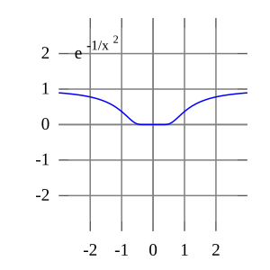
The function e ^{(−1/x two)} is non analytic at x = 0: the Taylor series is identically 0, although the role is non.

If f (x) is given by a convergent power series in an open deejay centred at b in the complex airplane (or an interval in the real line), it is said to exist analytic in this region. Thus for x in this region, f is given by a convergent ability series

${\displaystyle f(ten)=\sum _{north=0}^{\infty }a_{n}(x-b)^{north}.}$

Differentiating by x the above formula n times, then setting x = b gives:

${\displaystyle {\frac {f^{(n)}(b)}{n!}}=a_{north}}$

then the ability series expansion agrees with the Taylor series. Thus a function is analytic in an open up disk centred at b if and only if its Taylor serial converges to the value of the office at each point of the disk.

If f (x) is equal to the sum of its Taylor serial for all 10 in the complex plane, it is called entire. The polynomials, exponential function east ^x , and the trigonometric functions sine and cosine, are examples of entire functions. Examples of functions that are non unabridged include the foursquare root, the logarithm, the trigonometric office tangent, and its inverse, arctan. For these functions the Taylor series do not converge if x is far from b. That is, the Taylor series diverges at x if the altitude between x and b is larger than the radius of convergence. The Taylor series can be used to calculate the value of an entire function at every point, if the value of the function, and of all of its derivatives, are known at a unmarried point.

Uses of the Taylor series for analytic functions include:

1. The partial sums (the Taylor polynomials) of the serial can exist used equally approximations of the function. These approximations are expert if sufficiently many terms are included.
2. Differentiation and integration of power series can exist performed term by term and is hence specially piece of cake.
3. An analytic function is uniquely extended to a holomorphic function on an open disk in the circuitous plane. This makes the mechanism of complex analysis bachelor.
4. The (truncated) series can be used to compute function values numerically, (often by recasting the polynomial into the Chebyshev course and evaluating it with the Clenshaw algorithm).
5. Algebraic operations tin can exist done readily on the power serial representation; for case, Euler'due south formula follows from Taylor series expansions for trigonometric and exponential functions. This event is of fundamental importance in such fields as harmonic analysis.
6. Approximations using the first few terms of a Taylor series tin make otherwise unsolvable problems possible for a restricted domain; this approach is oftentimes used in physics.

Approximation error and convergence [edit]

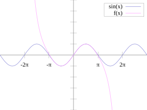
The sine role (bluish) is closely approximated by its Taylor polynomial of degree vii (pink) for a total period centered at the origin.

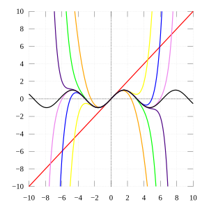
The Taylor polynomials for ln(1 + x) simply provide accurate approximations in the range −1 < x ≤ 1. For x > i, Taylor polynomials of higher caste provide worse approximations.

The Taylor approximations for ln(1 + x) (black). For ten > 1, the approximations diverge.

Pictured is an accurate approximation of sin 10 around the point x = 0. The pink curve is a polynomial of degree seven:

${\displaystyle \sin \left(x\correct)\approx x-{\frac {10^{3}}{iii!}}+{\frac {x^{5}}{5!}}-{\frac {x^{7}}{7!}}.\!}$

The error in this approximation is no more than | 10 |⁹ / 9!. For a full cycle centered at the origin (−π < x < π) the error is less than 0.08215. In particular, for −1 < 10 < 1, the error is less than 0.000003.

In dissimilarity, also shown is a picture of the natural logarithm function ln(one + x) and some of its Taylor polynomials around a = 0. These approximations converge to the function just in the region −1 < 10 ≤ 1; outside of this region the higher-degree Taylor polynomials are worse approximations for the function.

The mistake incurred in approximating a office past its nth-degree Taylor polynomial is called the remainder or residual and is denoted by the part R _n (x). Taylor'south theorem tin can exist used to obtain a bound on the size of the residue.

In general, Taylor series need not be convergent at all. And in fact the set of functions with a convergent Taylor serial is a meager set in the Fréchet infinite of polish functions. And even if the Taylor serial of a role f does converge, its limit demand not in general be equal to the value of the function f (x). For instance, the function

${\displaystyle f(10)={\begin{cases}e^{-1/ten^{2}}&{\text{if }}x\neq 0\\[3mu]0&{\text{if }}10=0\end{cases}}}$

is infinitely differentiable at x = 0, and has all derivatives zip there. Consequently, the Taylor series of f (ten) about x = 0 is identically cipher. Nonetheless, f (x) is not the goose egg function, so does not equal its Taylor series around the origin. Thus, f (x) is an example of a non-analytic smoothen office.

In real analysis, this example shows that there are infinitely differentiable functions f (x) whose Taylor series are not equal to f (ten) even if they converge. By contrast, the holomorphic functions studied in complex analysis always possess a convergent Taylor serial, and fifty-fifty the Taylor series of meromorphic functions, which might take singularities, never converge to a value different from the function itself. The complex function eastward ^{−1/z 2} , however, does not approach 0 when z approaches 0 forth the imaginary axis, then it is not continuous in the complex aeroplane and its Taylor serial is undefined at 0.

More generally, every sequence of real or circuitous numbers tin appear as coefficients in the Taylor series of an infinitely differentiable office defined on the existent line, a consequence of Borel's lemma. As a effect, the radius of convergence of a Taylor series tin exist naught. There are even infinitely differentiable functions divers on the real line whose Taylor series take a radius of convergence 0 everywhere.^[8]

A function cannot be written equally a Taylor serial centred at a singularity; in these cases, one tin often still reach a series expansion if ane allows also negative powers of the variable ten; come across Laurent series. For instance, f (x) = eastward ^{−one/x 2} tin be written every bit a Laurent series.

Generalization [edit]

There is, however, a generalization^{[9] [10]} of the Taylor series that does converge to the value of the function itself for any divisional continuous function on (0,∞), using the calculus of finite differences. Specifically, i has the following theorem, due to Einar Hille, that for whatever t > 0,

${\displaystyle \lim _{h\to 0^{+}}\sum _{north=0}^{\infty }{\frac {t^{n}}{n!}}{\frac {\Delta _{h}^{n}f(a)}{h^{north}}}=f(a+t).}$

Hither Δ ⁿ
_h is the nth finite difference operator with pace size h. The series is precisely the Taylor series, except that divided differences appear in identify of differentiation: the serial is formally similar to the Newton series. When the function f is analytic at a, the terms in the series converge to the terms of the Taylor series, and in this sense generalizes the usual Taylor serial.

In general, for whatsoever infinite sequence a _i , the following power series identity holds:

${\displaystyle \sum _{northward=0}^{\infty }{\frac {u^{due north}}{north!}}\Delta ^{n}a_{i}=due east^{-u}\sum _{j=0}^{\infty }{\frac {u^{j}}{j!}}a_{i+j}.}$

And so in particular,

${\displaystyle f(a+t)=\lim _{h\to 0^{+}}e^{-t/h}\sum _{j=0}^{\infty }f(a+jh){\frac {(t/h)^{j}}{j!}}.}$

The serial on the correct is the expectation value of f (a + X), where X is a Poisson-distributed random variable that takes the value jh with probability e ^−t/h · (t/h) ^j / j! . Hence,

${\displaystyle f(a+t)=\lim _{h\to 0^{+}}\int _{-\infty }^{\infty }f(a+x)dP_{t/h,h}(x).}$

The law of large numbers implies that the identity holds.^[11]

List of Maclaurin series of some mutual functions [edit]

Several important Maclaurin series expansions follow.^[12] All these expansions are valid for complex arguments x.

Exponential office [edit]

The exponential role e ^x (in blueish), and the sum of the first n + ane terms of its Taylor serial at 0 (in red).

The exponential function ${\displaystyle e^{x}}$ (with base of operations e) has Maclaurin series

${\displaystyle e^{x}=\sum _{n=0}^{\infty }{\frac {x^{n}}{n!}}=one+ten+{\frac {x^{two}}{2!}}+{\frac {x^{3}}{3!}}+\cdots }$ .

It converges for all x.

The exponential generating function of the Bell numbers is the exponential function of the predecessor of the exponential function:

${\displaystyle \exp[\exp(x)-1]=\sum _{north=0}^{\infty }{\frac {B_{n}}{north!}}x^{n}}$

Natural logarithm [edit]

The natural logarithm (with base of operations e) has Maclaurin serial

${\displaystyle {\begin{aligned}\ln(1-x)&=-\sum _{n=i}^{\infty }{\frac {ten^{n}}{n}}=-x-{\frac {x^{2}}{two}}-{\frac {x^{3}}{3}}-\cdots ,\\\ln(ane+x)&=\sum _{north=1}^{\infty }(-1)^{n+1}{\frac {ten^{north}}{north}}=x-{\frac {ten^{ii}}{two}}+{\frac {x^{3}}{iii}}-\cdots .\end{aligned}}}$

They converge for ${\displaystyle |x|<1}$ . (In addition, the series for ln(1 − x) converges for 10 = −one, and the series for ln(1 + x) converges for 10 = 1.)

Geometric series [edit]

The geometric series and its derivatives take Maclaurin series

${\displaystyle {\begin{aligned}{\frac {ane}{1-x}}&=\sum _{n=0}^{\infty }x^{n}\\{\frac {one}{(1-x)^{2}}}&=\sum _{n=i}^{\infty }nx^{due north-ane}\\{\frac {ane}{(1-x)^{3}}}&=\sum _{north=2}^{\infty }{\frac {(northward-one)due north}{2}}x^{n-2}.\stop{aligned}}}$

All are convergent for ${\displaystyle |x|<ane}$ . These are special cases of the binomial series given in the adjacent section.

Binomial series [edit]

The binomial series is the ability series

$${\displaystyle (1+x)^{\alpha }=\sum _{northward=0}^{\infty }{\binom {\alpha }{n}}x^{n}}$$

whose coefficients are the generalized binomial coefficients

$${\displaystyle {\binom {\alpha }{n}}=\prod _{k=i}^{north}{\frac {\alpha -m+1}{k}}={\frac {\alpha (\alpha -ane)\cdots (\blastoff -n+1)}{due north!}}.}$$

(If n = 0, this production is an empty product and has value 1.) It converges for ${\displaystyle |10|<1}$ for any real or complex number α.

When α = −1, this is essentially the infinite geometric series mentioned in the previous department. The special cases α = 1 / ii and α = − ane / 2 give the square root function and its inverse:

$${\displaystyle {\begin{aligned}(ane+x)^{\frac {1}{2}}&=1+{\tfrac {one}{ii}}x-{\tfrac {1}{viii}}10^{2}+{\tfrac {one}{16}}10^{3}-{\tfrac {5}{128}}10^{4}+{\tfrac {seven}{256}}x^{five}-\cdots &&=\sum _{n=0}^{\infty }{\frac {(-1)^{n-1}(2n)!}{iv^{northward}(n!)^{2}(2n-i)}}x^{n},\\(1+10)^{-{\frac {1}{two}}}&=1-{\tfrac {1}{two}}x+{\tfrac {3}{8}}x^{2}-{\tfrac {5}{xvi}}x^{3}+{\tfrac {35}{128}}ten^{4}-{\tfrac {63}{256}}x^{5}+\cdots &&=\sum _{n=0}^{\infty }{\frac {(-1)^{n}(2n)!}{iv^{n}(n!)^{2}}}ten^{northward}.\end{aligned}}}$$

When but the linear term is retained, this simplifies to the binomial approximation.

Trigonometric functions [edit]

The usual trigonometric functions and their inverses accept the post-obit Maclaurin series:

${\displaystyle {\begin{aligned}\sin ten&=\sum _{n=0}^{\infty }{\frac {(-1)^{n}}{(2n+ane)!}}x^{2n+1}&&=10-{\frac {x^{3}}{3!}}+{\frac {x^{v}}{5!}}-\cdots &&{\text{for all }}x\\[6pt]\cos x&=\sum _{n=0}^{\infty }{\frac {(-1)^{n}}{(2n)!}}x^{2n}&&=1-{\frac {x^{two}}{2!}}+{\frac {x^{4}}{4!}}-\cdots &&{\text{for all }}x\\[6pt]\tan ten&=\sum _{n=1}^{\infty }{\frac {B_{2n}(-four)^{n}\left(1-iv^{n}\correct)}{(2n)!}}x^{2n-1}&&=x+{\frac {x^{3}}{3}}+{\frac {2x^{5}}{15}}+\cdots &&{\text{for }}|x|<{\frac {\pi }{2}}\\[6pt]\sec x&=\sum _{n=0}^{\infty }{\frac {(-1)^{n}E_{2n}}{(2n)!}}x^{2n}&&=ane+{\frac {10^{two}}{2}}+{\frac {5x^{four}}{24}}+\cdots &&{\text{for }}|x|<{\frac {\pi }{2}}\\[6pt]\arcsin x&=\sum _{n=0}^{\infty }{\frac {(2n)!}{4^{north}(northward!)^{2}(2n+1)}}x^{2n+1}&&=x+{\frac {x^{3}}{6}}+{\frac {3x^{five}}{forty}}+\cdots &&{\text{for }}|x|\leq 1\\[6pt]\arccos x&={\frac {\pi }{2}}-\arcsin x\\&={\frac {\pi }{2}}-\sum _{n=0}^{\infty }{\frac {(2n)!}{4^{due north}(n!)^{ii}(2n+1)}}ten^{2n+ane}&&={\frac {\pi }{2}}-x-{\frac {ten^{3}}{half-dozen}}-{\frac {3x^{5}}{40}}-\cdots &&{\text{for }}|x|\leq 1\\[6pt]\arctan x&=\sum _{n=0}^{\infty }{\frac {(-1)^{n}}{2n+1}}x^{2n+one}&&=x-{\frac {x^{iii}}{three}}+{\frac {x^{5}}{5}}-\cdots &&{\text{for }}|x|\leq one,\ x\neq \pm i\cease{aligned}}}$

All angles are expressed in radians. The numbers B₁₀₀₀ actualization in the expansions of tan ten are the Bernoulli numbers. The E _{one thousand} in the expansion of sec 10 are Euler numbers.

Hyperbolic functions [edit]

The hyperbolic functions have Maclaurin series closely related to the series for the corresponding trigonometric functions:

${\displaystyle {\begin{aligned}\sinh x&=\sum _{n=0}^{\infty }{\frac {x^{2n+1}}{(2n+1)!}}&&=ten+{\frac {x^{3}}{3!}}+{\frac {10^{five}}{five!}}+\cdots &&{\text{for all }}x\\[6pt]\cosh x&=\sum _{n=0}^{\infty }{\frac {x^{2n}}{(2n)!}}&&=1+{\frac {x^{2}}{2!}}+{\frac {10^{4}}{4!}}+\cdots &&{\text{for all }}10\\[6pt]\tanh x&=\sum _{northward=1}^{\infty }{\frac {B_{2n}4^{northward}\left(4^{north}-ane\right)}{(2n)!}}x^{2n-1}&&=x-{\frac {x^{3}}{iii}}+{\frac {2x^{5}}{fifteen}}-{\frac {17x^{seven}}{315}}+\cdots &&{\text{for }}|x|<{\frac {\pi }{ii}}\\[6pt]\operatorname {arsinh} x&=\sum _{north=0}^{\infty }{\frac {(-1)^{n}(2n)!}{4^{n}(n!)^{2}(2n+1)}}x^{2n+1}&&=x-{\frac {x^{three}}{six}}+{\frac {3x^{five}}{forty}}-\cdots &&{\text{for }}|x|\leq 1\\[6pt]\operatorname {artanh} 10&=\sum _{northward=0}^{\infty }{\frac {ten^{2n+ane}}{2n+1}}&&=x+{\frac {x^{three}}{three}}+{\frac {x^{five}}{5}}+\cdots &&{\text{for }}|x|\leq one,\ x\neq \pm ane\finish{aligned}}}$

The numbers B_yard actualization in the series for tanh ten are the Bernoulli numbers.

Polylogarithmic functions [edit]

The polylogarithms accept these defining identities:

${\displaystyle {\text{Li}}_{2}(x)=\sum _{n=1}^{\infty }{\frac {1}{n^{ii}}}x^{n}}$

${\displaystyle {\text{Li}}_{iii}(10)=\sum _{n=1}^{\infty }{\frac {1}{n^{iii}}}ten^{north}}$

The Legendre chi functions are divers as follows:

${\displaystyle \chi _{2}(x)=\sum _{n=0}^{\infty }{\frac {1}{(2n+i)^{2}}}x^{2n+1}}$

${\displaystyle \chi _{3}(x)=\sum _{northward=0}^{\infty }{\frac {i}{(2n+one)^{3}}}ten^{2n+one}}$

And the formulas presented below are called inverse tangent integrals:

${\displaystyle {\text{Ti}}_{2}(x)=\sum _{n=0}^{\infty }{\frac {(-one)^{due north}}{(2n+1)^{2}}}x^{2n+one}}$

${\displaystyle {\text{Ti}}_{3}(10)=\sum _{n=0}^{\infty }{\frac {(-1)^{northward}}{(2n+1)^{3}}}x^{2n+i}}$

In statistical thermodynamics these formulas are of great importance.

Elliptic functions [edit]

The complete elliptic integrals of start kind K and of second kind E can be defined as follows:

${\displaystyle {\frac {ii}{\pi }}Yard(x)=\sum _{northward=0}^{\infty }{\frac {[(2n)!]^{two}}{xvi^{north}(n!)^{4}}}x^{2n}}$

${\displaystyle {\frac {2}{\pi }}E(x)=\sum _{n=0}^{\infty }{\frac {[(2n)!]^{2}}{(one-2n)16^{northward}(north!)^{4}}}x^{2n}}$

The Jacobi theta functions draw the earth of the elliptic modular functions and they take these Taylor series:

${\displaystyle \vartheta _{00}(ten)=1+2\sum _{n=one}^{\infty }x^{n^{ii}}}$

${\displaystyle \vartheta _{01}(x)=one+two\sum _{n=1}^{\infty }(-one)^{n}ten^{northward^{2}}}$

The regular partition number sequence P(n) has this generating role:

${\displaystyle \vartheta _{00}(x)^{-1/6}\vartheta _{01}(x)^{-2/iii}{\biggl [}{\frac {\vartheta _{00}(10)^{iv}-\vartheta _{01}(10)^{4}}{16\,10}}{\biggr ]}^{-1/24}=\sum _{northward=0}^{\infty }P(north)x^{north}=\prod _{thousand=ane}^{\infty }{\frac {ane}{one-x^{k}}}}$

The strict partition number sequence Q(n) has that generating function:

${\displaystyle \vartheta _{00}(10)^{one/half-dozen}\vartheta _{01}(x)^{-1/3}{\biggl [}{\frac {\vartheta _{00}(x)^{four}-\vartheta _{01}(x)^{four}}{16\,ten}}{\biggr ]}^{i/24}=\sum _{n=0}^{\infty }Q(northward)x^{n}=\prod _{k=ane}^{\infty }{\frac {1}{1-x^{2k-i}}}}$

Calculation of Taylor series [edit]

Several methods exist for the calculation of Taylor series of a big number of functions. One tin attempt to use the definition of the Taylor series, though this often requires generalizing the form of the coefficients according to a readily apparent pattern. Alternatively, 1 can use manipulations such as substitution, multiplication or partition, addition or subtraction of standard Taylor serial to construct the Taylor series of a office, by virtue of Taylor series being power series. In some cases, ane can also derive the Taylor series past repeatedly applying integration past parts. Particularly user-friendly is the utilise of computer algebra systems to calculate Taylor series.

First example [edit]

In gild to compute the 7th degree Maclaurin polynomial for the part

${\displaystyle f(x)=\ln(\cos x),\quad x\in \left(-{\frac {\pi }{2}},{\frac {\pi }{2}}\right)}$ ,

one may first rewrite the office as

${\displaystyle f(x)=\ln {\bigl (}1+(\cos 10-1){\bigr )}\!}$ .

The Taylor serial for the natural logarithm is (using the big O note)

${\displaystyle \ln(1+x)=ten-{\frac {10^{2}}{2}}+{\frac {x^{3}}{iii}}+{O}\left(x^{4}\right)\!}$

and for the cosine part

${\displaystyle \cos x-1=-{\frac {10^{ii}}{ii}}+{\frac {x^{4}}{24}}-{\frac {10^{6}}{720}}+{O}\left(10^{8}\right)\!}$ .

The latter serial expansion has a zilch abiding term, which enables united states of america to substitute the 2d serial into the first one and to hands omit terms of college order than the 7th degree past using the big O notation:

${\displaystyle {\begin{aligned}f(x)&=\ln {\bigl (}1+(\cos x-1){\bigr )}\\&=(\cos 10-i)-{\tfrac {1}{2}}(\cos x-1)^{2}+{\tfrac {one}{3}}(\cos x-1)^{3}+{O}\left((\cos 10-1)^{4}\right)\\&=\left(-{\frac {10^{two}}{2}}+{\frac {x^{iv}}{24}}-{\frac {10^{6}}{720}}+{O}\left(x^{eight}\right)\right)-{\frac {i}{ii}}\left(-{\frac {x^{2}}{2}}+{\frac {x^{4}}{24}}+{O}\left(x^{six}\right)\right)^{ii}+{\frac {i}{iii}}\left(-{\frac {x^{2}}{ii}}+O\left(x^{4}\correct)\right)^{3}+{O}\left(x^{viii}\right)\\&=-{\frac {x^{2}}{2}}+{\frac {x^{4}}{24}}-{\frac {x^{6}}{720}}-{\frac {ten^{4}}{8}}+{\frac {x^{six}}{48}}-{\frac {x^{six}}{24}}+O\left(x^{8}\right)\\&=-{\frac {x^{ii}}{two}}-{\frac {x^{4}}{12}}-{\frac {10^{6}}{45}}+O\left(x^{8}\right).\end{aligned}}\!}$

Since the cosine is an even function, the coefficients for all the odd powers ten, ten ^three, ten ^five, x ⁷, ... have to be zero.

2d instance [edit]

Suppose we want the Taylor series at 0 of the function

${\displaystyle g(x)={\frac {e^{x}}{\cos ten}}.\!}$

We have for the exponential function

${\displaystyle e^{x}=\sum _{n=0}^{\infty }{\frac {ten^{n}}{due north!}}=1+x+{\frac {ten^{2}}{2!}}+{\frac {x^{three}}{iii!}}+{\frac {x^{iv}}{4!}}+\cdots \!}$

and, as in the starting time example,

${\displaystyle \cos x=1-{\frac {10^{2}}{2!}}+{\frac {x^{iv}}{four!}}-\cdots \!}$

Assume the power series is

${\displaystyle {\frac {eastward^{x}}{\cos x}}=c_{0}+c_{1}x+c_{two}x^{2}+c_{iii}10^{3}+\cdots \!}$

And then multiplication with the denominator and commutation of the series of the cosine yields

${\displaystyle {\begin{aligned}e^{x}&=\left(c_{0}+c_{one}ten+c_{two}10^{2}+c_{iii}x^{three}+\cdots \correct)\cos x\\&=\left(c_{0}+c_{1}x+c_{2}x^{2}+c_{3}x^{3}+c_{iv}x^{4}+\cdots \correct)\left(i-{\frac {x^{ii}}{2!}}+{\frac {x^{4}}{4!}}-\cdots \right)\\&=c_{0}-{\frac {c_{0}}{ii}}x^{2}+{\frac {c_{0}}{4!}}ten^{4}+c_{1}x-{\frac {c_{one}}{2}}10^{3}+{\frac {c_{ane}}{four!}}10^{5}+c_{2}10^{two}-{\frac {c_{2}}{two}}10^{iv}+{\frac {c_{2}}{4!}}ten^{vi}+c_{3}x^{3}-{\frac {c_{3}}{2}}10^{5}+{\frac {c_{3}}{4!}}x^{7}+c_{4}x^{4}+\cdots \end{aligned}}\!}$

Collecting the terms up to fourth guild yields

${\displaystyle e^{x}=c_{0}+c_{1}x+\left(c_{two}-{\frac {c_{0}}{2}}\right)x^{2}+\left(c_{3}-{\frac {c_{one}}{2}}\right)x^{3}+\left(c_{4}-{\frac {c_{2}}{two}}+{\frac {c_{0}}{iv!}}\right)x^{4}+\cdots \!}$

The values of ${\displaystyle c_{i}}$ can be found by comparing of coefficients with the superlative expression for ${\displaystyle e^{x}}$ , yielding:

${\displaystyle {\frac {due east^{x}}{\cos x}}=1+x+x^{2}+{\frac {2x^{3}}{iii}}+{\frac {ten^{iv}}{ii}}+\cdots .\!}$

3rd case [edit]

Here nosotros employ a method chosen "indirect expansion" to expand the given function. This method uses the known Taylor expansion of the exponential office. In order to expand (1 + ten)e^x as a Taylor series in x, we utilize the known Taylor series of part east ^x :

${\displaystyle e^{x}=\sum _{n=0}^{\infty }{\frac {x^{north}}{n!}}=1+x+{\frac {x^{2}}{2!}}+{\frac {x^{iii}}{3!}}+{\frac {ten^{4}}{4!}}+\cdots .}$

Thus,

${\displaystyle {\begin{aligned}(ane+10)e^{x}&=eastward^{10}+xe^{x}=\sum _{north=0}^{\infty }{\frac {10^{n}}{n!}}+\sum _{northward=0}^{\infty }{\frac {x^{north+one}}{n!}}=i+\sum _{n=1}^{\infty }{\frac {10^{n}}{n!}}+\sum _{n=0}^{\infty }{\frac {ten^{n+1}}{n!}}\\&=1+\sum _{n=1}^{\infty }{\frac {x^{n}}{n!}}+\sum _{n=1}^{\infty }{\frac {10^{due north}}{(north-1)!}}=1+\sum _{n=one}^{\infty }\left({\frac {1}{n!}}+{\frac {1}{(n-1)!}}\right)x^{n}\\&=1+\sum _{northward=one}^{\infty }{\frac {n+i}{n!}}10^{n}\\&=\sum _{n=0}^{\infty }{\frac {n+one}{north!}}ten^{n}.\end{aligned}}}$

Taylor series equally definitions [edit]

Classically, algebraic functions are defined by an algebraic equation, and transcendental functions (including those discussed to a higher place) are defined by some property that holds for them, such as a differential equation. For example, the exponential function is the role which is equal to its own derivative everywhere, and assumes the value 1 at the origin. However, one may as well define an analytic function by its Taylor series.

Taylor series are used to ascertain functions and "operators" in various areas of mathematics. In particular, this is truthful in areas where the classical definitions of functions break downwardly. For case, using Taylor series, one may extend analytic functions to sets of matrices and operators, such as the matrix exponential or matrix logarithm.

In other areas, such equally formal analysis, it is more convenient to work directly with the power series themselves. Thus one may define a solution of a differential equation as a ability series which, i hopes to prove, is the Taylor serial of the desired solution.

Taylor serial in several variables [edit]

The Taylor serial may also be generalized to functions of more than ane variable with^{[13] [xiv]}

${\displaystyle {\brainstorm{aligned}T(x_{one},\ldots ,x_{d})&=\sum _{n_{i}=0}^{\infty }\cdots \sum _{n_{d}=0}^{\infty }{\frac {(x_{i}-a_{ane})^{n_{i}}\cdots (x_{d}-a_{d})^{n_{d}}}{n_{1}!\cdots n_{d}!}}\,\left({\frac {\partial ^{n_{i}+\cdots +n_{d}}f}{\partial x_{ane}^{n_{1}}\cdots \partial x_{d}^{n_{d}}}}\right)(a_{one},\ldots ,a_{d})\\&=f(a_{1},\ldots ,a_{d})+\sum _{j=ane}^{d}{\frac {\fractional f(a_{ane},\ldots ,a_{d})}{\partial x_{j}}}(x_{j}-a_{j})+{\frac {ane}{2!}}\sum _{j=1}^{d}\sum _{yard=ane}^{d}{\frac {\partial ^{2}f(a_{1},\ldots ,a_{d})}{\partial x_{j}\fractional x_{yard}}}(x_{j}-a_{j})(x_{grand}-a_{chiliad})\\&\qquad \qquad +{\frac {one}{three!}}\sum _{j=1}^{d}\sum _{k=1}^{d}\sum _{l=1}^{d}{\frac {\partial ^{three}f(a_{1},\ldots ,a_{d})}{\partial x_{j}\partial x_{k}\partial x_{fifty}}}(x_{j}-a_{j})(x_{k}-a_{one thousand})(x_{l}-a_{l})+\cdots \end{aligned}}}$

For example, for a part ${\displaystyle f(x,y)}$ that depends on two variables, 10 and y, the Taylor series to 2d guild near the point (a, b) is

${\displaystyle f(a,b)+(x-a)f_{x}(a,b)+(y-b)f_{y}(a,b)+{\frac {i}{2!}}{\Big (}(x-a)^{2}f_{20}(a,b)+2(10-a)(y-b)f_{xy}(a,b)+(y-b)^{two}f_{yy}(a,b){\Big )}}$

where the subscripts denote the respective fractional derivatives.

A second-gild Taylor series expansion of a scalar-valued function of more one variable tin be written compactly as

${\displaystyle T(\mathbf {ten} )=f(\mathbf {a} )+(\mathbf {x} -\mathbf {a} )^{\mathsf {T}}Df(\mathbf {a} )+{\frac {i}{2!}}(\mathbf {x} -\mathbf {a} )^{\mathsf {T}}\left\{D^{2}f(\mathbf {a} )\right\}(\mathbf {x} -\mathbf {a} )+\cdots ,}$

where D f (a) is the gradient of f evaluated at x = a and D ² f (a) is the Hessian matrix. Applying the multi-index notation the Taylor series for several variables becomes

${\displaystyle T(\mathbf {10} )=\sum _{|\blastoff |\geq 0}{\frac {(\mathbf {x} -\mathbf {a} )^{\alpha }}{\alpha !}}\left({\mathrm {\fractional } ^{\blastoff }}f\right)(\mathbf {a} ),}$

which is to be understood as a still more than abbreviated multi-alphabetize version of the first equation of this paragraph, with a full analogy to the single variable example.

Example [edit]

2d-order Taylor series approximation (in orangish) of a part f (x,y) = e^x ln(1 + y) around the origin.

In lodge to compute a 2d-order Taylor series expansion around bespeak (a, b) = (0, 0) of the office

${\displaystyle f(x,y)=east^{ten}\ln(ane+y),}$

i first computes all the necessary fractional derivatives:

${\displaystyle {\begin{aligned}f_{10}&=e^{10}\ln(i+y)\\[6pt]f_{y}&={\frac {e^{ten}}{i+y}}\\[6pt]f_{xx}&=east^{x}\ln(1+y)\\[6pt]f_{yy}&=-{\frac {e^{10}}{(ane+y)^{2}}}\\[6pt]f_{xy}&=f_{yx}={\frac {east^{10}}{ane+y}}.\end{aligned}}}$

Evaluating these derivatives at the origin gives the Taylor coefficients

${\displaystyle {\begin{aligned}f_{10}(0,0)&=0\\f_{y}(0,0)&=i\\f_{20}(0,0)&=0\\f_{yy}(0,0)&=-one\\f_{xy}(0,0)&=f_{yx}(0,0)=1.\finish{aligned}}}$

Substituting these values in to the general formula

${\displaystyle {\begin{aligned}T(x,y)=&f(a,b)+(x-a)f_{x}(a,b)+(y-b)f_{y}(a,b)\\&{}+{\frac {1}{2!}}\left((ten-a)^{ii}f_{xx}(a,b)+2(x-a)(y-b)f_{xy}(a,b)+(y-b)^{two}f_{yy}(a,b)\correct)+\cdots \end{aligned}}}$

produces

${\displaystyle {\brainstorm{aligned}T(x,y)&=0+0(x-0)+ane(y-0)+{\frac {1}{2}}{\Big (}0(x-0)^{two}+ii(10-0)(y-0)+(-1)(y-0)^{two}{\Big )}+\cdots \\&=y+xy-{\frac {y^{ii}}{two}}+\cdots \end{aligned}}}$

Since ln(1 + y) is analytic in | y | < 1, nosotros take

${\displaystyle e^{10}\ln(1+y)=y+xy-{\frac {y^{2}}{2}}+\cdots ,\qquad |y|<ane.}$

Comparison with Fourier series [edit]

The trigonometric Fourier serial enables i to limited a periodic function (or a function divers on a closed interval [a,b]) as an infinite sum of trigonometric functions (sines and cosines). In this sense, the Fourier series is analogous to Taylor series, since the latter allows one to limited a function equally an infinite sum of powers. Notwithstanding, the two serial differ from each other in several relevant bug:

• The finite truncations of the Taylor series of f (x) about the point 10 = a are all exactly equal to f at a . In contrast, the Fourier series is computed by integrating over an entire interval, so in that location is generally no such bespeak where all the finite truncations of the series are verbal.
• The computation of Taylor series requires the knowledge of the function on an arbitrary small neighbourhood of a point, whereas the ciphering of the Fourier series requires knowing the function on its whole domain interval. In a certain sense one could say that the Taylor series is "local" and the Fourier serial is "global".
• The Taylor series is divers for a function which has infinitely many derivatives at a single point, whereas the Fourier series is defined for whatever integrable office. In particular, the function could be nowhere differentiable. (For example, f (10) could be a Weierstrass function.)
• The convergence of both series has very unlike backdrop. Even if the Taylor series has positive convergence radius, the resulting series may non coincide with the office; but if the function is analytic then the series converges pointwise to the function, and uniformly on every compact subset of the convergence interval. Concerning the Fourier serial, if the part is foursquare-integrable then the series converges in quadratic mean, merely additional requirements are needed to ensure the pointwise or uniform convergence (for instance, if the function is periodic and of form C¹ and so the convergence is uniform).
• Finally, in practice ane wants to approximate the function with a finite number of terms, say with a Taylor polynomial or a partial sum of the trigonometric series, respectively. In the case of the Taylor serial the error is very small in a neighbourhood of the point where it is computed, while it may be very large at a afar bespeak. In the case of the Fourier series the error is distributed along the domain of the office.

See too [edit]

• Asymptotic expansion
• Generating role
• Laurent series
• Madhava series
• Newton's divided divergence interpolation
• Padé approximant
• Puiseux series
• Shift operator

Notes [edit]

1. ^ Thomas & Finney 1996, §8.ix
2. ^ Lindberg, David (2007). The Beginnings of Western Science (2nd ed.). University of Chicago Press. p. 33. ISBN978-0-226-48205-7.
3. ^ Kline, G. (1990). Mathematical Idea from Aboriginal to Modern Times . New York: Oxford University Press. pp. 35–37. ISBN0-19-506135-7.
4. ^ Boyer, C.; Merzbach, U. (1991). A History of Mathematics (Second revised ed.). John Wiley and Sons. pp. 202–203. ISBN0-471-09763-2.
5. ^ "Neither Newton nor Leibniz – The Pre-History of Calculus and Angelic Mechanics in Medieval Kerala" (PDF). MAT 314. Canisius College. Archived (PDF) from the original on 2015-02-23. Retrieved 2006-07-09 .
6. ^ S. G. Dani (2012). "Aboriginal Indian Mathematics – A Conspectus". Resonance. 17 (3): 236–246. doi:10.1007/s12045-012-0022-y. S2CID 120553186.
7. ^ Taylor, Brook (1715). Methodus Incrementorum Directa et Inversa [Direct and Opposite Methods of Incrementation] (in Latin). London. p. 21–23 (Prop. VII, Thm. 3, Cor. 2). Translated into English in Struik, D. J. (1969). A Source Volume in Mathematics 1200–1800. Cambridge, Massachusetts: Harvard Academy Press. pp. 329–332.
8. ^ Rudin, Walter (1980), Real and Complex Analysis, New Delhi: McGraw-Loma, p. 418, Exercise 13, ISBN0-07-099557-5
9. ^ Feller, William (1971), An introduction to probability theory and its applications, Book 2 (3rd ed.), Wiley, pp. 230–232 .
10. ^ Hille, Einar; Phillips, Ralph S. (1957), Functional assay and semi-groups, AMS Colloquium Publications, vol. 31, American Mathematical Lodge, pp. 300–327 .
11. ^ Feller, William (1970). An introduction to probability theory and its applications. Vol. two (3 ed.). p. 231.
12. ^ Most of these can be found in (Abramowitz & Stegun 1970).
13. ^ Lars Hörmander (1990), The analysis of fractional differential operators, volume 1, Springer, Eqq. 1.i.seven and i.i.vii′
14. ^ Duistermaat; Kolk (2010), Distributions: Theory and applications, Birkhauser, ch. 6

References [edit]

• Abramowitz, Milton; Stegun, Irene A. (1970), Handbook of Mathematical Functions with Formulas, Graphs, and Mathematical Tables, New York: Dover Publications, Ninth printing
• Thomas, George B. Jr.; Finney, Ross 50. (1996), Calculus and Analytic Geometry (9th ed.), Addison Wesley, ISBN0-201-53174-7
• Greenberg, Michael (1998), Advanced Applied science Mathematics (2nd ed.), Prentice Hall, ISBN0-thirteen-321431-1

External links [edit]

• "Taylor series", Encyclopedia of Mathematics, EMS Press, 2001 [1994]
• Weisstein, Eric W. "Taylor Series". MathWorld.

Taylor Series Ln 1 X,

Source: https://en.wikipedia.org/wiki/Taylor_series

Posted by: mitchellmovence.blogspot.com

Share this post